MuZero - part 1
General ·MuZero: A high level view
The previous post on the AlphaZero (AZ) algorithm served mainly as warm-up. It helped to build an intuition for Monte Carlo tree search (MCTS) and how this powerful heuristic jives well with neural networks. Even more interesting, however, I find MuZero (MZ; original paper). The MZ algorithm (or at least its pseudocode) has been out for a while, so I’ll keep the recap brief. I’d like to touch on some key difference with respect to AZ and how I decided to implement. This post concerns a simple version intended to start with, while the following post will focus on scaling. That should provide a good base to explore some potential MZ applications I’ve had in mind.
Overview
Crucially, MZ foregoes any direct access to an (environmental) simulator. Whereas AZ uses this simulator to search future trajectories via MCTS, MZ instead relies on a state embedding to perform MCTS in latent space. This has interesting implications for high-dimension state-spaces (e.g. in vision) by enabling search through a lower-dimensional embedding. The embedding is unconstrained and by training end-to-end it can be used in whatever way the neural net sees fit.
 |
|---|
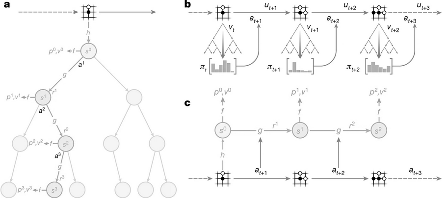
| From Schrittweiser et al., visualizing MZ’s search (a), environment interaction (b), and training (c). |
The algorithm relies on three networks:
- $s^{k=0} = h(o_t; \theta_f)$: representation network, where the current environment is observed ($o_t$) and passed through $f$ to provide the initial embedding $s_0$.
- $p^k, v^k = f(s^k; \theta_h)$: prediction network, which evaluates an embedding and estimates its value as well as proposes a policy $p_k$ over actions.
- $s^k, r^k = g(s^{k-1}, a^k; \theta_g)$: dynamics network, modeling the state transitions and associated reward of embeddings. Depending on the problem, it can be useful to use a recurrent network here. However, in Markovian settings a feed-forward model suffices and is what I rely on here.
Interaction with the environment can then proceed as follows:
- Observe the current environment
- Generate its embedding with representation function $h$.
- Perform MCTS by recurrently relying on dynamics function $g$ for the roll-out of states and prediction function $f$ to do value and policy estimation.
- Take an action based on the visit counts generated by MCTS.
Episodes of such interactions are saved to allow for offline-training. A trajectory is sampled from the replay buffer and first the observation is fed into $h$. We can then unroll the model at each step $k$ for $K$ steps with $g$ by feeding in the previous hidden state $s^k$ and real action $a_{t+k}$. The set of parameters ${\theta_f, \theta_h, \theta_g}$ are trained via back-prop simultaneously and end-to-end1. To do so, the policy suggestion $p^k$ generated by $f$ is aligned with the policy $\pi_{t+k}$ provided by the MCTS procedure. Meanwhile, $v^k \approx z_{t+k}$ and $r^k \approx u_{t+k}$ with $z_{t+k}$ as the sample return which is simply the final reward for board games (in which case $u_{t+k}=0$ due to absence of intermediate rewards). The latent state can thus come represent whatever is relevant to achieve this. Finally, the complete loss, including L2 regularization, looks as follows:
\[\large l_t(\theta) = \sum^K_{k=0} l^p (\pi_{t+k},p_t^k) + \sum^K_{k=0} l^v(z_{t+k},v_t^k) + \sum_{k=1}^K l^r (u_{t+k},r_t^k) + c \Vert \theta \Vert ^2\]Moving from A(Z) to (M)Z
Concretely, inside the MCTS some important changes were made. For example, each time we expand a node, we rely on dynamics function $g$ to provide the associated next state:
def expand(self, turn, prior, dynamics):

    self.expanded = True
    # 1. generate child
    # 2. assign priors

    prior = prior[self.legal_moves]

    # add Dirichlet-noise
    noise = np.random.dirichlet([self.dir_alpha]*len(prior))
    prior = prior*(1-self.dir_frac) + noise*self.dir_frac
    prior /= np.sum(prior)

    for i, a in enumerate(prior):

        a_oh = F.one_hot(torch.tensor(self.legal_moves[i]), num_classes=9).float()
        next_state, _ = dynamics.predict(torch.cat([self.embedded_state, a_oh.view(1,-1)], dim=1))
        self.child[i] = Node(torch.tensor(next_state), turn*-1, self.legal_moves, self.dir_alpha, self.dir_frac)
        self.child[i].prior = prior[i].item()
Note that the Dirichlet-noise constitutes a heuristic which corrupts the prior. This functions as an exploration incentive and can help distribute the probability mass across the different actions, thereby promoting action selection stochasticity.
Further, due to the lack of access to an explicit simulator, MZ cannot rely on it to know whether the tree search has reaching a terminal state. While it makes the initial observation and can determine which moves are legal at that moment, it is not bound by the game once it starts its search in latent space. This is resolved during training, where terminal states (and any subsequent ones) are treated as absorbing states. As planning beyond terminal states should generally result in poor performance, pure reward-based learning appears to sufficiently address the issue.
idx_absorb = idx.copy() # indices corrected for absorbing states
id_k_list = [idx.copy()] # list of indices for each step k
NAB_list = [] # records whether a state is absorbing (inverse Boolean for easy indexing)

for k in range(self.K):

    # check for absorbing states
    not_absorb = ((state_log[idx+1+k,:]==0).sum(axis=1) != 9)

    if k == 0:
        idx_bool_either = not_absorb.copy()
    else: # after k=0 we need to check if current or any preceding state is absorbing
        idx_bool_either = [ x and y for (x,y) in zip(not_absorb, NAB_list[-1])]

    idx_absorb[idx_bool_either] += 1 # only indices for non-absorbing states are incremented by 1

    NAB_list.append(idx_bool_either.copy())
    id_k_list.append(idx_absorb.copy())
Otherwise, MZ is a true successor to AZ as it relies on much of the same principles. Feel free to check out the preliminary code here. With all the basic functionality in place, I’m looking forward to scaling this up in the upcoming weeks!
-
PyTorch makes this very easy: you can include the different models (here
dynamics,prediction, andrepresentation) in the optimizer as follows:dynamics = DynamicsNet().to(self.device) prediction = PredictionNet().to(self.device) representation = RepresentationNet().to(self.device) opt = torch.optim.SGD(list(dynamics.parameters()) + list(prediction.parameters()) + list(representation.parameters()), lr=lr, weight_decay=1e-5)